7 Week 7: Scatterplots
7.1 Goals
- You’ll learn how to visualise the relationship between two continuous variables in a scatterplot.
- You’ll gain some experience with summarising and manipulating large datasets.
7.2 Summarising datasets
Vanhove (2014) investigated how people’s ability to
recognise written and spoken cognates in a related but
unknown language develops throughout the lifespan and
how it is related to linguistic and cognitive factors.
The dataset Vanhove2014_Translations.csv contains the
raw data of this study. For each of the 163 participants,
this dataset contains 100 entries (one for each cognate),
for a total of 16,300 rows.
Each translation was rated as correct or incorrect.
Additionally, the dataset contains some information
about the participants (e.g., their performance on other
tasks) as well as about the stimuli (e.g., a measure
expressing its formal similarity to its French, German or English cognate).
## Rows: 16300 Columns: 15
## ── Column specification ────────────────────────────
## Delimiter: ","
## chr  (5): Stimulus, Mode, Translation, Sex, Status
## dbl (10): Subject, Trial, Correct, Age, NrLang, DS.Total, WST.Right, Raven.R...
##
## ℹ Use `spec()` to retrieve the full column specification for this data.
## ℹ Specify the column types or set `show_col_types = FALSE` to quiet this message.
The variables:
Stimulus: The word to be translated.Subject: The participant’s ID.Mode: Whether the word was presented in its spoken (Auditory) or in its written form (Visual).Trial: The position of the word in the task.Translation: The participant’s translation attempt for the stimulus.Correct: Whether the translation was correct (1) or incorrect (0).SexAgeNrLang: The number of languages the participant spoken.DS.Total: The participant’s score on a working memory task.WST.Right: The participant’s score on a German vocabulary test.Raven.Right: The participant’s score on an intelligence test.English.Total: The participant’s score on an English-language test.Status: Whether the stimulus has a German, English, or French cognates (target) or not (profile).MinLev: The degree of formal discrepancy between the stimulus and its most similar German, English or French cognate. (lower = more similar)
Missing values were labelled NA (not available).
A rough summary can be obtained like so:
##    Stimulus            Subject         Mode               Trial
##  Length:16300       Min.   :  64   Length:16300       Min.   : 1.0
##  Class :character   1st Qu.:2909   Class :character   1st Qu.:13.0
##  Mode  :character   Median :5731   Mode  :character   Median :25.5
##                     Mean   :5317                      Mean   :25.5
##                     3rd Qu.:7794                      3rd Qu.:38.0
##                     Max.   :9913                      Max.   :50.0
##
##  Translation           Correct           Sex                 Age
##  Length:16300       Min.   :0.0000   Length:16300       Min.   :10.00
##  Class :character   1st Qu.:0.0000   Class :character   1st Qu.:16.00
##  Mode  :character   Median :0.0000   Mode  :character   Median :39.00
##                     Mean   :0.3523                      Mean   :40.28
##                     3rd Qu.:1.0000                      3rd Qu.:60.00
##                     Max.   :1.0000                      Max.   :86.00
##
##      NrLang         DS.Total        WST.Right      Raven.Right
##  Min.   :1.000   Min.   : 2.000   Min.   : 4.00   Min.   : 0.0
##  1st Qu.:2.000   1st Qu.: 5.000   1st Qu.:29.00   1st Qu.:12.0
##  Median :3.000   Median : 6.000   Median :34.00   Median :19.0
##  Mean   :3.067   Mean   : 6.374   Mean   :30.24   Mean   :17.8
##  3rd Qu.:4.000   3rd Qu.: 8.000   3rd Qu.:36.00   3rd Qu.:24.0
##  Max.   :9.000   Max.   :12.000   Max.   :41.00   Max.   :35.0
##                                   NA's   :100
##  English.Total      Status              MinLev
##  Min.   : 3.00   Length:16300       Min.   :0.0000
##  1st Qu.:20.75   Class :character   1st Qu.:0.2857
##  Median :31.00   Mode  :character   Median :0.4000
##  Mean   :28.30                      Mean   :0.4566
##  3rd Qu.:37.00                      3rd Qu.:0.6062
##  Max.   :44.00                      Max.   :1.0000
##  NA's   :300
In order to be able to sensibly visualise these data, we need to first transform this dataset. If we’re interested in the relationship between the participants’ age, sex, and linguistic and cognitive test results on the one hand and their translation performance on the other hand, it seems useful to first compute the number of correct translations for spoken and written words per participant. There are a couple of ways you could do this in R; I find the method outlined below the most transparent one.
Let’s start with a simple example. We’ll first compute the total number of correct responses in the entire dataset. The comments show you how you can read the R code out loud.
# 1st attempt: Total number of correct answers

# Take object 'd' (our dataset), then
d |>
  # summarise it as follows:
  # - compute the sum of 'Correct' and call this sum 'number_correct'
  summarise(number_correct = sum(Correct))
## # A tibble: 1 × 1
## number_correct
## <dbl>
## 1 5743The result is shown in the console. We can also
save it as a separate object so that we can
work with it later. Here I save it as an object
called overall_accuracy:
(To type the symbol combination |> (known as the pipe; read out loud as ‘and then’), you can also use the shortcut ctrl + shift + m.)
The total number of correct answers in the entire dataset isn’t too useful to us: we need the number of correct answers per participant.
# 2nd attempt: Number of correct answers per participant

# Create new object 'per_part' as follows:
# take 'd', and then...
per_part <- d |>
  # group it by Subject, and then...
  group_by(Subject)  |>
  # compute the sum of Correct within each group
  summarise(number_correct = sum(Correct))

# Show result
per_part
## # A tibble: 163 × 2
## Subject number_correct
## <dbl> <dbl>
## 1 64 49
## 2 78 39
## 3 134 36
## 4 230 38
## 5 288 21
## 6 326 45
## 7 447 47
## 8 527 24
## 9 545 33
## 10 550 46
## # ℹ 153 more rowsNow we have the total number of correct translations per participant, but this figure contains both the responses to written and to spoken words. It’d be more useful to split this figure up by modality:
# 3rd attempt: Number of correct translations per participant,
# split up by modality.

per_part2 <- d |>
  # group by Subject and Mode
  group_by(Subject, Mode) |>
  summarise(number_correct = sum(Correct))
## `summarise()` has grouped output by 'Subject'. You
## can override using the `.groups` argument.## # A tibble: 326 × 3
## # Groups: Subject [163]
## Subject Mode number_correct
## <dbl> <chr> <dbl>
## 1 64 Auditory 24
## 2 64 Visual 25
## 3 78 Auditory 19
## 4 78 Visual 20
## 5 134 Auditory 24
## 6 134 Visual 12
## 7 230 Auditory 12
## 8 230 Visual 26
## 9 288 Auditory 12
## 10 288 Visual 9
## # ℹ 316 more rowsThe message (summarise() has grouped output by ‘Subject’.) isn’t harmful, but you can get rid of it as follows:
per_part2 <- d |>
  group_by(Subject, Mode) |>
  summarise(number_correct = sum(Correct),
            .groups = "drop")
Our goal is to visualise the relationship between variables such as IQ, age, and L1 vocabulary skills on the one hand and the participants’ translation performance on the other hand. To do this, we need to add these variable to the summary. Again, there are several ways to do this; here’s one.
# 4th attempt: Like above, but adding Age, etc.

# Create a new object with participant-related information.
# Take 'd', and then...
part_info <- d |>
  # Select the following columns
  select(Subject, Age, Sex, WST.Right,
         Raven.Right, English.Total,
         NrLang, DS.Total)
Like d, part_info consists of 16,300 rows.
But each row is repeated 100 times.
Using distinct(), the duplicates are deleted:
Now we can add the information from part_info to per_part2:
# Create new object 'per_part3'.
# Take object 'per_part2', and then...
per_part3 <- per_part2 |>
  # join it with 'part_info' using 'Subject' as the "zipper"
  full_join(part_info, by = "Subject")

# Show result
per_part3
## # A tibble: 326 × 10
## Subject Mode number_correct Age Sex WST.Right Raven.Right English.Total
## <dbl> <chr> <dbl> <dbl> <chr> <dbl> <dbl> <dbl>
## 1 64 Audit… 24 27 fema… 34 28 42
## 2 64 Visual 25 27 fema… 34 28 42
## 3 78 Audit… 19 47 fema… 33 26 27
## 4 78 Visual 20 47 fema… 33 26 27
## 5 134 Audit… 24 33 male 32 24 24
## 6 134 Visual 12 33 male 32 24 24
## 7 230 Audit… 12 84 male 37 20 31
## 8 230 Visual 26 84 male 37 20 31
## 9 288 Audit… 12 28 male 35 24 39
## 10 288 Visual 9 28 male 35 24 39
## # ℹ 316 more rows
## # ℹ 2 more variables: NrLang <dbl>, DS.Total <dbl>One final problem remains: The number of correct answers
includes responses to both cognates and to non-cognates.
We’re only interested in the responses to cognates, however.
Using filter(), we only retain the responses that are of interest:
# 5th attempt: Like above, but only consider target stimuli.
per_part <- d |>
  # only consider target stimuli
  filter(Status == "target") |>
  # group by Subject and Mode
  group_by(Subject, Mode) |>
  # Compute sum of Correct
  summarise(number_correct = sum(Correct),
            .groups = "drop") |>
  # Add the information from part_info using Subject as the "zipper"
  full_join(part_info, by = "Subject")
per_part
## # A tibble: 326 × 10
## Subject Mode number_correct Age Sex WST.Right Raven.Right English.Total
## <dbl> <chr> <dbl> <dbl> <chr> <dbl> <dbl> <dbl>
## 1 64 Audit… 23 27 fema… 34 28 42
## 2 64 Visual 25 27 fema… 34 28 42
## 3 78 Audit… 19 47 fema… 33 26 27
## 4 78 Visual 20 47 fema… 33 26 27
## 5 134 Audit… 24 33 male 32 24 24
## 6 134 Visual 12 33 male 32 24 24
## 7 230 Audit… 12 84 male 37 20 31
## 8 230 Visual 26 84 male 37 20 31
## 9 288 Audit… 12 28 male 35 24 39
## 10 288 Visual 9 28 male 35 24 39
## # ℹ 316 more rows
## # ℹ 2 more variables: NrLang <dbl>, DS.Total <dbl>7.3 Scatterplots
To investigate the relationhip between, say, WST.Right and number_correct,
we can plot these data in a scatterplot. While we’re at it, we can split up
this graph into two panels: one for written words, and one for spoken words.
ggplot(dat = per_part,
       aes(x = WST.Right,
           y = number_correct)) +
  # Incidentally, you can specify the shape and colour of the points yourself.
  geom_point(shape = 21, colour = "darkblue", fill = "green") +
  # Type in "colours()" to see which colour names are recognised by R.
  # Type in ?pch to see which 'shape' values are accepted.
  xlab("L1 vocabulary test") +
  ylab("Number of correct translations\n(out of 45)") +
  facet_grid(cols = vars(Mode)) +
  labs(title = "A title of your choice",
       subtitle = "(and perhaps even a subtitle)",
       caption = "(and a caption)")
## Warning: Removed 2 rows containing missing values or values
## outside the scale range (`geom_point()`).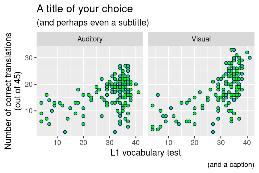
(The warning concerns missing values in the WST variable. Inspect the dataset
to find for how many participants the WST score is missing!)
As we’ll discuss in class, scatterplots are the indispensable first (and sometimes final) step when analysing the relationship between two continuous variables.
As for the decision which variable to put along which axis. By and large, put the variable that is most likely to be the cause of the relationship along the x axis and the variable that is most likely to be the effect along the y axis. In this case, it seems more likely that L1 skills affect one’s ability to recognise cognates in a foreign language than vice versa. Hence, put the variable representing L1 skills along the x axis.
7.4 Exercise
Draw a scatterplot that shows the relationship between the participants’ score on the English-language test and the number of correct translations. How many participants’ data are shown?
Hand in the compiled HTML report. Mention the number of participants whose data are shown in the R code.