A quick introduction to Gaussian process regression

For my Master’s thesis in statistics, I took a closer look at a method that allows you to do predictive regression modelling when the inputs are represented as probability distributions.

1. Predictive model, here: for solving regression problems.

2. Goal: explain basic logic.

The goal of this blog post is to introduce the nuts and bolts of Gaussian process regression.

Assume that for any finite collection of outputs \(Y_1, \dots, Y_n\), the vector \(\boldsymbol{Y} = (Y_1, \dots, Y_n)^{\top}\) has an \(n\)-variate Gaussian (i.e., Normal) distribution: \[\boldsymbol Y \sim \mathcal{N}_n(\boldsymbol \mu, \boldsymbol \Sigma),\] where \(\boldsymbol \mu\) is the distribution’s \(n\)-valued mean vector and \(\boldsymbol \Sigma\) is its \(n \times n\) covariance matrix.

For simplicity, we assume that the mean vector of this distribution is \(\boldsymbol{0}\). The \((i,j)\)-th element of \(\boldsymbol \Sigma\) expresses the covariance of the \(i\)-th and \(j\)-th element of \(\boldsymbol Y\).

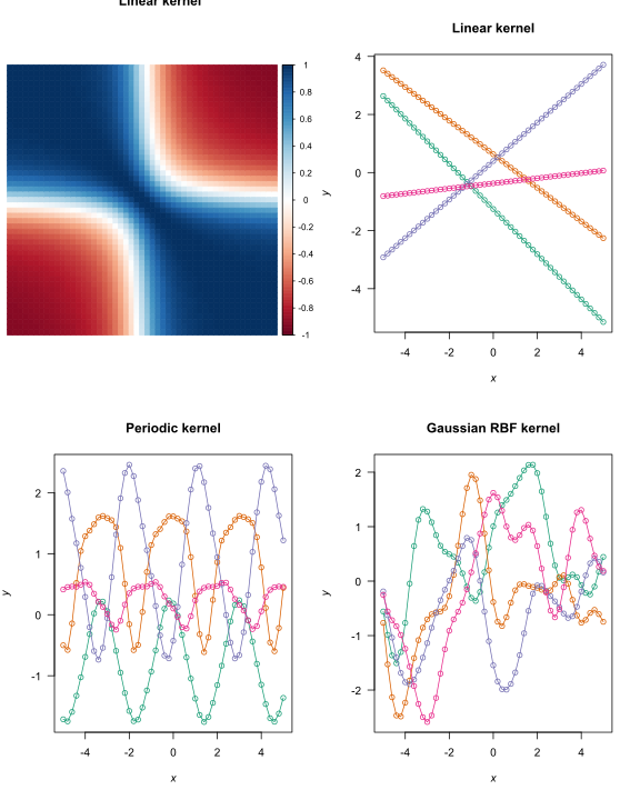
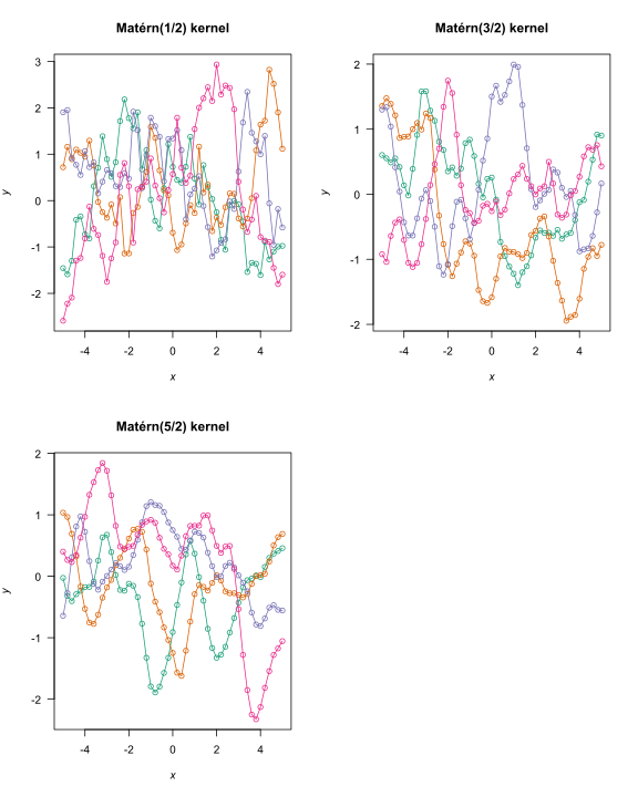
# Plotting functions -----------------------------------------------------------
plot_gpr <- function(x, K, n = 4, main = "") {
  cols <- RColorBrewer::brewer.pal(n, "Dark2")
  Y <- MASS::mvrnorm(n = n, mu = rep(0, length(x)), Sigma = K)
  plot(x = x, y = Y[1, ], ylim = range(Y), type = "n", las = 1,
     xlab = expression(italic(x)), 
     ylab = expression(italic(y)), 
     main = main)
  for (i in seq_len(n)) {
    points(x = x, y = Y[i, ], type = "o", col = cols[i])
  }
}
plot_corr <- function(K, main = "") {
  corrplot::corrplot(cov2cor(K),
    method = "color", title = main, tl.pos = "n")
}

# Plot kernels -----------------------------------------------------------------
op <- par(no.readonly = TRUE)
par(mfrow = c(2, 2))

# Random seed
set.seed(2026-07-07)

# Predictor data and distances between them
x <- seq(-5, 5, by = 0.2)
D <- outer(x, x, "-") |> abs()

# Linear kernel with an offset
K_linear <- outer(x, x, "*") + matrix(1, nrow = length(x), ncol = length(x))
plot_corr(K_linear, main = "Linear kernel")
plot_gpr(x, K_linear, main = "Linear kernel")

# Periodic kernel
K_periodic <- exp(-sin(D)^2)
plot_gpr(x, K_periodic, main = "Periodic kernel")

# RBF kernel
K_rbf <- exp(-D^2)
plot_gpr(x, K_rbf, main = "Gaussian RBF kernel")

# Matérn 1/2 kernel
K_matern12 <- exp(-D)
plot_gpr(x, K_matern12, main = "Matérn(1/2) kernel")

# Matérn 3/2 kernel
K_matern32 <- (1 + sqrt(3) * D) * exp(-sqrt(3)*D)
plot_gpr(x, K_matern32, main = "Matérn(3/2) kernel")

# Matérn 5/2 kernel
K_matern52 <- (1 + sqrt(5) * D + 5 * D^2 / 3) * exp(-sqrt(5)*D)
plot_gpr(x, K_matern52, main = "Matérn(5/2) kernel")

par(op)

Figure 1: A scatterplot to which we want to add a trend line.

Figure 2: A scatterplot to which we want to add a trend line.

References and further reading

Session info

devtools::session_info("attached")

Warning in system2("quarto", "-V", stdout = TRUE, env = paste0("TMPDIR=", :
running command '"quarto"
TMPDIR=C:/Users/VanhoveJ/AppData/Local/Temp/Rtmpi4kf6j/file986acf401f -V' had
status 1

─ Session info ───────────────────────────────────────────────────────────────
 setting  value
 version  R version 4.5.0 (2025-04-11 ucrt)
 os       Windows 11 x64 (build 26200)
 system   x86_64, mingw32
 ui       RTerm
 language (EN)
 collate  English_United Kingdom.utf8
 ctype    English_United Kingdom.utf8
 tz       Europe/Zurich
 date     2026-07-09
 pandoc   3.1.1 @ C:/Program Files/RStudio/resources/app/bin/quarto/bin/tools/ (via rmarkdown)
 quarto   NA @ C:\\Users\\VanhoveJ\\AppData\\Local\\Programs\\Quarto\\bin\\quarto.exe

──────────────────────────────────────────────────────────────────────────────