Different distributions, same boxplot

When I want to compare the distribution of some more or less continuous variable between two or more groups, the boxplot is my default graph of choice. In the absence of outliers, they compactly summarise a distribution in five numbers: the minimum, first quartile, median, third quartile, and maximum.¹ They avoid arbitrary choices such as histogram binning and kernel choice and, unlike kernel density plots, they don’t assume that the underlying distribution is smooth.

But boxplots can also be deceptive. One important reason for this is that two distributions can be represented by the same boxplot yet be qualitatively different. This is why I encourage students and colleagues to overlay the individual data points when using boxplots, as this helps to ward off some common misinterpretations and may reveal some additional structure in the data.

To further drive this point home, I thought it’d be useful to have an R function that can generate quite radically different distributions that would produce identical boxplots—in much the same way that I wrote a function that outputs different bivariate distributions yielding the same correlation coefficient (What data patterns can lie behind a correlation coefficient?).

R functions

The first code snippet defines such a function, boxplot_data(). It takes, among other inputs, a desired minimum, first quartile, median, third quartile, and maximum, and generates data conforming to this five-number summary. The parameter k governs the number of data points in the distribution, and the other parameters regulate what the distribution looks like in the intervals determined by the five-number summary.

boxplot_data <- function(
    k,                          
    q0, q1, q2, q3, q4,    
    gaps = rep(0, 3),                 
    shapes = rep("uniform", 4), 
    margins_lo = c(0.05, 0.05, 0.05, 0.05),
    margins_hi = c(0.05, 0.05, 0.05, 0.05)) {
  # Generate univariate data whose five-number summary matches 
  # specified values. Data between these values follows user-specified
  # distributions.
  
  # k: Integer, k >= 2. Generates n = 4*k observations.
  # q0, q1, q2, q3, q4: Desired five-number summary in ascending order:
  #                     q0 = minimum, q1 = first hinge, q2 = median,
  #                     q3 = second hinge, q4 = maximum.
  #                     If q0 or q4 lies too far from the q1 or q3,
  #                     these values will be overridden with a message.
  # gaps: Numeric vector (length 3) controlling the gaps around q1, q2, and q3. 
  #       If gaps[1] = 1, the closest data point near q1 is as far away from q1 as possible;
  #       If gaps[1] = 0, at least two data points lie on q1.
  #       gaps[2] and gaps[3] regulate the gaps between the data and q2, q3.
  #       gap should be a vector in [0,1]^3 such that gaps[1] + gaps[2] <= 1
  #       and gaps[2] + gaps[3] <= 1. Otherwise, the values will be overridden
  #       with a message.
  # shapes: Character vector (length 4) specifying the distribution shape in each interval.
  # margins_lo, margins_hi: Numeric vectors (length 4) giving lower and upper insets 
  #                         (proportions) that keep generated values 
  #                         away from the interval endpoints.

  if (k < 2) stop("k must be >= 2")
  n <- 4 * k
  
  desired <- c(q0, q1, q2, q3, q4)
  if (any(desired != sort(desired))) {
    stop("five-number summary must be in ascending order.")
  }
  if (q0 < q1 - 1.5*(q3 - q1)) {
    q0 <- q1 - 1.5*(q3 - q1)
    message(paste0("Desired minimum too low. Set to ", q0, "."))
  }
  if (q4 > q3 + 1.5*(q3 - q1)) {
    q4 <- q3 + 1.5*(q3 - q1)
    message(paste0("Desired maximum too high. Set to ", q4, "."))
  }
  
  # Squish values into [0,1]
  squish <- function(x) {
    x <- x - min(x)
    if (isTRUE(all.equal(max(x), 0))) return(x)
    x <- x / max(x)
  }
  if (min(gaps) < 0 | max(gaps) > 1) {
    gaps <- squish(gaps)
    message(paste0("Gap values outside of permissible range. Set to ", gaps, "."))
  }
  if (gaps[1] + gaps[2] > 1) {
    gaps[c(1,2)] <- gaps[c(1,2)] / sum(gaps[c(1,2)])
    message(paste0("First and second gap values incompatible. Set to ", gaps[c(1,2)], "."))
  }
  if (gaps[2] + gaps[3] > 1) {
    gaps[c(2,3)] <- gaps[c(2,3)] / sum(gaps[c(2,3)])
    message(paste0("Second and third gap values incompatible. Set to ", gaps[c(2,3)], "."))
  }
  
  if (min(margins_lo) < 0 | max(margins_lo) > 1) {
    margins_lo <- squish(margins_lo)
    message(paste0("Margin-low values outside of permissible range. Set to ", margins_lo, "."))
  }
  if (min(margins_hi) < 0 | max(margins_hi) > 1) {
    margins_hi <- squish(margins_hi)
    message(paste0("Margin-high values outside of permissible range. Set to ", margins_hi, "."))
  }
  for (i in seq_along(margins_lo)) {
    if (margins_lo[i] + margins_hi[i] > 1) {
      m_lo <- margins_lo[i] / (margins_lo[i] + margins_hi[i])
      m_hi <- margins_hi[i] / (margins_lo[i] + margins_hi[i])
      margins_lo[i] <- m_lo
      margins_hi[i] <- m_hi
      message(paste0("Margin values for segment ", i, " incompatible. Set to ", m_lo, " and ", m_hi, "."))
    }
  }
  
  # Compute symmetric gaps around hinges and median:
  s <- numeric(3)
  s[1] <- gaps[1] * min(q1 - q0, q2 - q1)
  s[2] <- gaps[2] * min(q2 - q1, q3 - q2)
  s[3] <- gaps[3] * min(q3 - q2, q4 - q3)
    
  data <- numeric(n)
  data[1]       <- q0
  data[k]       <- q1 - s[1] # gap around first hinge
  data[k + 1]   <- q1 + s[1]
  data[2 * k]   <- q2 - s[2] # gap around median
  data[2*k + 1] <- q2 + s[2]
  data[3 * k]   <- q3 - s[3] # gap around second hinge
  data[3*k + 1] <- q3 + s[3]
  data[n]       <- q4

  # Distributions within segments
  right_skewed <- function(m) {
    x <- abs(rnorm(m))
    squish(x)
  }
  left_skewed <- function(m) {
    x <- 1 - right_skewed(m)
    squish(x)
  }
  one_bump <- function(m) {
    x <- rnorm(m)
    squish(x)
  }
  two_bumps <- function(m) {
    x <- c(rnorm(floor(m/2), -2), rnorm(ceiling(m/2), 2))
    squish(x)
  }
  
  fill_segment <- function(v0, v1, m, shape, a0, b0) {
    if (m <= 0) return(numeric(0))
    u <- switch(shape,
                uniform    = runif(m),
                right_skew = right_skewed(m),
                left_skew  = left_skewed(m),
                one_bump   = one_bump(m),
                two_bumps  = two_bumps(m),
                stop("unknown shape: ", shape)
    )
    u <- a0 + (1 - a0 - b0) * u
    sort(v0 + (v1 - v0) * u)
  }
  
  # Obtain bounds for segments
  seg_bounds <- list(c(1, k), c(k+1, 2*k), c(2*k+1, 3*k), c(3*k+1, n))
  for (j in seq_along(seg_bounds)) {
    i0 <- seg_bounds[[j]][1]
    i1 <- seg_bounds[[j]][2]
    m <- i1 - i0 - 1
    if (m <= 0) next
    pts <- fill_segment(data[i0], data[i1], m, shapes[j], a0 = margins_lo[j], b0 = margins_hi[j])
    data[(i0 + 1):(i1 - 1)] <- pts
  }
  
  if (isFALSE(all.equal(fivenum(data), desired))) {
    warning("Not exact match with desired values.")
  }
  
  data
}

NoteHow boxplot_data() works

The most important inputs to the boxplot_data() function are the desired locations of the distribution’s minimum (q0) and maximum (q4) as well as the location of the hinges (q1, q3) and the median (q2). The function will generate a distribution such that, if you use R’s boxplot() function, the boxplot’s box and whiskers will match these values. The desired number of data points is k multiplied by 4.

The gaps parameter governs how far away from the first hinge, the median and the second hinge, respectively, the closest data points may be, relatively speaking. For instance, if gaps = c(0, 0, 0), then there will be actual data points corresponding to the first hinge, the median and the second hinge. If gaps = c(1, 1, 1), then the data points will lie as far away from these hinges and the median as possible. If gaps = c(0, 1, 0), some data points will coincide with the first and third hinge, but no data point will match the median. (The exception is when the median itself coincides with the first or second hinge.) The red brackets in Figure 1 illustrate the meaning of the gaps parameter; a wide gap was chosen around the median, a narrow gap around the first hinge, and a medium gap around the second hinge.

draw_boxplot_structure <- function(
    q0, q1, q2, q3, q4,
    gaps = c(.3, .2, .3),
    margins_lo = c(.05, .05, .05, .05),
    margins_hi = c(.05, .05, .05, .05))
{
  # This function was first written by Copilot Basic.
  # I then edited it.
  s1 <- gaps[1] * min(q1 - q0, q2 - q1)
  s2 <- gaps[2] * min(q2 - q1, q3 - q2)
  s3 <- gaps[3] * min(q3 - q2, q4 - q3)
  
  plot(
    0, 0,
    type = "n",
    xlim = c(0, 10),
    ylim = c(q0 - .1 * (q4 - q0),
             q4 + .1 * (q4 - q0)),
    xaxt = "n",
    yaxt = "n",
    xlab = "",
    ylab = ""
  )
  
  abline(h = q0, lty = 3, col = "lightgrey")
  abline(h = q1, lty = 3, col = "lightgrey")
  abline(h = q2, lty = 3, col = "lightgrey")
  abline(h = q3, lty = 3, col = "lightgrey")
  abline(h = q4, lty = 3, col = "lightgrey")
  
  axis(2)
  
  cols <- c(
    "#008cba",
    "#008cba",
    "#008cba",
    "#008cba"
  )
  
  # ---------- BOXPLOT ----------
  xbox <- 7.5
  bw <- 0.8
  
  rect(
    xbox - bw/2, q1,
    xbox + bw/2, q3,
    col = "white",
    border = "black",
    lwd = 2
  )
  
  segments(xbox, q0, xbox, q1, lwd = 2)
  segments(xbox, q3, xbox, q4, lwd = 2)
  
  segments(xbox - bw/4, q0,
           xbox + bw/4, q0, lwd = 2)
  
  segments(xbox - bw/4, q4,
           xbox + bw/4, q4, lwd = 2)
  
  segments(
    xbox - bw/2, q2,
    xbox + bw/2, q2,
    lwd = 3
  )
  
  text(
    rep(xbox + 0.9, 5),
    c(q0, q1, q2, q3, q4),
    labels = c("q0", "q1", "q2", "q3", "q4"),
    pos = 4
  )
  
  # ---------- CONSTRUCTION DIAGRAM ----------
  
  xc <- 3
  
  segments(xc, q0, xc, q4, lwd = 1)
  
  segs <- list(
    c(q0,      q1 - s1),
    c(q1 + s1, q2 - s2),
    c(q2 + s2, q3 - s3),
    c(q3 + s3, q4)
  )
  
  for(i in 1:4){
    
    lo <- segs[[i]][1]
    hi <- segs[[i]][2]
    
    rect(
      xc - 0.5, lo,
      xc + 0.5, hi,
      col = cols[i],
      border = NA
    )
    
    rng <- hi - lo
    
    ml <- lo + margins_lo[i] * rng
    mh <- hi - margins_hi[i] * rng
    
    rect(
      xc - 0.5, lo,
      xc + 0.5, ml,
      col = "#ffa500",
      border = NA
    )
    
    rect(
      xc - 0.5, mh,
      xc + 0.5, hi,
      col = "#ffa500",
      border = NA
    )
    
    text(
      xc - 1.5,
      (lo + hi)/2,
      paste("segment", i),
      cex = .8
    )
  }
  
  # ---------- GAP BRACKETS ----------
  
  draw_gap <- function(y1, y2, x = 4.2, lab){
    
    arrows(
      x, y1,
      x, y2,
      code = 3,
      angle = 90,
      length = .08,
      col = "darkred",
      lwd = 2
    )
    
    text(
      x + 0.8,
      mean(c(y1, y2)),
      lab,
      col = "darkred"
    )
  }
  
  draw_gap(q1 - s1, q1 + s1, lab = "gap[1]")
  draw_gap(q2 - s2, q2 + s2, lab = "gap[2]")
  draw_gap(q3 - s3, q3 + s3, lab = "gap[3]")
  
  # ---------- HINGE / MEDIAN LABELS ----------
  
  points(
    rep(xc, 8),
    c(q1 - s1, q1 + s1,
      q2 - s2, q2 + s2,
      q3 - s3, q3 + s3,
      q0, q4),
    pch = 19
  )
  
  mtext(
    "Construction of data generated by boxplot_data()",
    side = 3,
    line = 0.5
  )
  
  legend(
    "bottomleft",
    inset=c(0,-0.2),
    xpd = TRUE,
    fill = c(cols[1], "#ffa500"),
    legend = c(
      "fill these regions with additional data (distribution controlled by shapes)",
      "no further data in these regions (excluded by margins)"
    ),
    bty = "n"
  )
  

}
par(las = 1)
draw_boxplot_structure(
  q0 = 0,
  q1 = 10,
  q2 = 20,
  q3 = 35,
  q4 = 50,
  gaps = c(.1, .6, .2),
  margins_lo = c(.3, .5, 0, 0),
  margins_hi = c(0, 0, 0, .8)
)

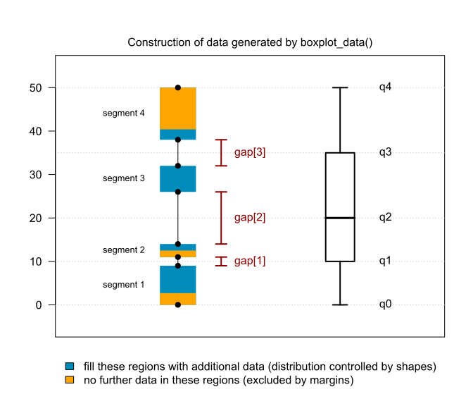
Figure 1: Explanation of how boxplot_data() works.

Through this process, the position of eight data points is determined: the minimum, the maximum, and two data points governing the position of the hinges and the median. These points define four segments:

• the segment between the minimum and the lowest closest neighbour to the first hinge;
• the segment between the upper closest neighbour to the first hinge and the lower closest neighbour to the median;
• the segment between the upper closest neighbour to the median and the lower closest neighbour to the second hinge;
• the segment between the upper closest neighbour to the second hinge and the maximum.

Each of these segments must be filled by \((4k - 8)/4 = k - 2\) observations. In principle, this can be done completely arbitrarily, and the new observations may, in principle, coincide with the segment boundaries. Three parameters allow us to control the distribution of the data in these segments.

• The shapes parameter governs the shape of the distribution in each segment. The function currently accepts uniform, left_skew, right_skew, one_bump and two_bumps for a uniform, left skewed, right skewed, centred unimodal and bimodal distribution, respectively. Adding other types of distribution is pretty easy. The distribution shape can be set separately for each segment.
• The margins_lo parameter specifies how near the data points may lie to the closest upper neighbours to the minimum, first hinge, median, and second hinge. That is, it specifies the margin from the lower ends of the segments. These margins are specified in relative terms, with margins_lo = c(0, 0, 0, 0) meaning that other data points may coincide with all upper neighbours and margins_lo = c(1, 1, 1, 1) meaning that no other data points may lie in the interior of the segments.
• The margins_hi parameter similarly specifies how near the data points may lie to the closest lower neighbours to the first hinge, the median, the second hinge, and the maximum. That is, it specifies the margin from the upper ends of the segments. In Figure 1, non-zero margins_lo values were specified for the minimum and the first hinge, and a non-zero margins_hi value was specified for the maximum.

If the values for the desired boxplot statistics or the gaps and margins_* parameters are badly specified, the function will attempt to rectify the problem and will output a message. The function does not allow you to generate data corresponding to a boxplot with outliers, but you can add these manually. This will change the position of the boxplot, though, but if you generate multiple datasets for the same boxplot statistics but with different underlying distributions, adding the same outliers to each dataset should still generate identical boxplots.

In the next snippet, I define the function draw_boxplots(), which uses boxplot_data() to generate six datasets with identical five-number summaries and then plots them. By default, 60 data points (4 * k, with k = 15) are generated for each dataset.

draw_boxplots <- function(k = 15, five_numbers = c(0, 7, 13, 27, 55), 
  show_mean = TRUE, show_data = FALSE, mfrow = c(3, 2), mar = c(1, 3, 4.1, 1), las = 1, ...) {
  # Plot 6 identical boxplots with different underlying distributions.
  
  draw_boxplot <- function(x, show_mean = TRUE, main = NULL) {
    boxplot(x, main = main, at = 1)
    points(x = jitter(rep(1, length(x)), 4), y = x)
    if (show_mean) points(x = 1, mean(x), col = "darkred", pch = 8, cex = 1.8)
  }
  
  five_numbers <- sort(five_numbers)
  q0 <- five_numbers[1]
  q1 <- five_numbers[2]
  q2 <- five_numbers[3]
  q3 <- five_numbers[4]
  q4 <- five_numbers[5]
  
  if (q0 < q1 - 1.5*(q3 - q1)) {
    q0 <- q0 - 1.5*(q3 - q1)
    warning(paste0("Minimum value too far from box. Was reset to ", q0, "."))
  }
  if (q4 > q3 + 1.5*(q3 - q1)) {
    q4 <- q3 + 1.5*(q3 - q1)
    warning(paste0("Maximum value too far from box. Was reset to ", q4, "."))
  }

  op <- par(no.readonly = TRUE)
  par(mfrow = mfrow, mar = mar, las = las, ...)
  
  # Spread out
  d1 <- boxplot_data(k, q0, q1, q2, q3, q4)
  draw_boxplot(d1, main = "Spread out data")
  
  # Gap around median
  d2 <- boxplot_data(k, q0, q1, q2, q3, q4,  
    shapes = c("left_skew", "right_skew", "left_skew", "right_skew"),
    gaps = c(0, 0.85, 0))
  draw_boxplot(d2, main = "Gap around median")
  
  # Five numbers typical
  lo <- rbinom(4, 1, 0.5)
  hi <- 1 - lo
  d3 <- boxplot_data(k, q0, q1, q2, q3, q4,  
    gaps = rep(0, 3),
    margins_lo = lo,
    margins_hi = hi)
  draw_boxplot(d3, main = "Only data at five numbers")
  
  # All quartiles atypical
  lo <- rbinom(4, 1, 0.5)
  hi <- 1 - lo
  d4 <- boxplot_data(k, q0, q1, q2, q3, q4,  
    gaps = rep(0.5, 3),
    margins_lo = lo,
    margins_hi = hi)
  draw_boxplot(d4, main = "Quartiles atypical")
  
  # 5) Nearly empty box
  d5 <- boxplot_data(k, q0, q1, q2, q3, q4,
    gaps = c(0, 1, 0),
    margins_lo = c(0, 0, 1, 0),
    margins_hi = c(0, 1, 0, 0))
  draw_boxplot(d5, main = "Nearly empty box")
  
  # 6) Nearly empty whiskers
  d6 <- boxplot_data(k, q0, q1, q2, q3, q4,  
    shapes = c("uniform", "left_skew", "right_skew", "uniform"),
    gaps = c(0, 0, 0),
    margins_lo = c(1, 0, 0, 0),
    margins_hi = c(0, 0, 0, 1))
  draw_boxplot(d6, main = "Nearly empty whiskers")
  
  par(op)
  
  if (show_data) {
    d <- data.frame(
      x = c(d1, d2, d3, d4, d5, d6),
      plot = rep(1:6, each = 4*k)
    )
    return(d)
  }
}

Examples

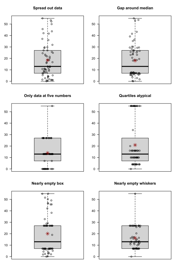
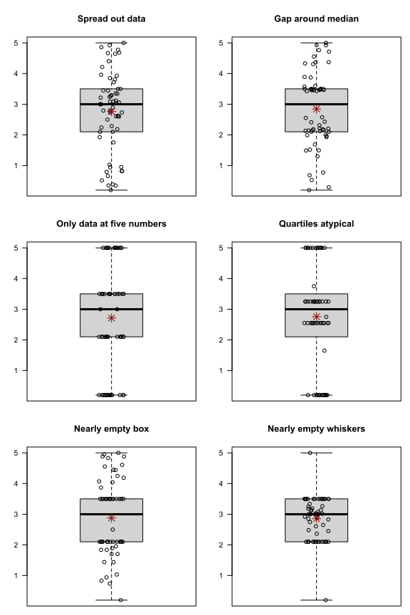
Figure 2 shows six boxplots, with the individual data points overlaid, that are obtained when using the default settings.

• The top row shows a distribution where the median is a pretty typical value (left) and a bimodal distribution in which the observations lie far from the median (right).
• The middle row shows a distribution that only has values at the five numbers (left) and a multimodal distribution in which none of the modes are centred around these five numbers (right).
• In the bottom row, either the box is pretty much empty (left), or the whiskers are pretty much empty (right).

draw_boxplots()

Figure 2: Six distributions with identical boxplots but with different underlying distributions. The red stars show the distributions’ means.

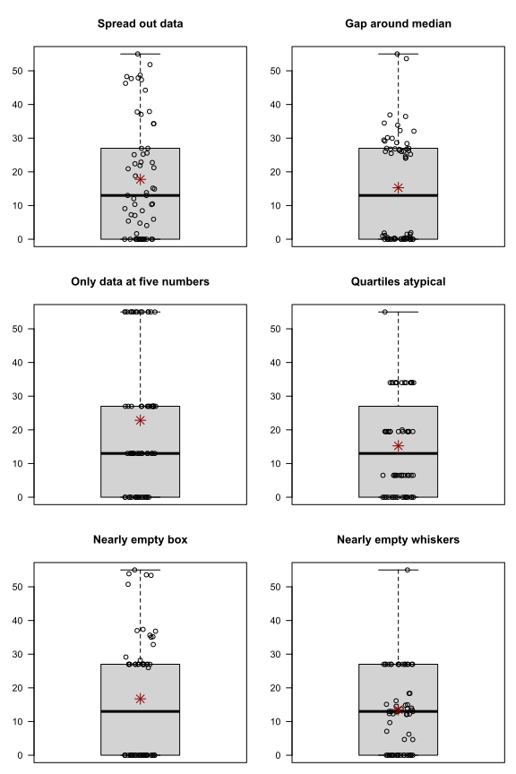
Figure 3 shows a similar line-up of boxplots, but this time, they are all degenerate: the first quartile and the minimum coincide.

draw_boxplots(five_numbers = c(0, 0, 13, 27, 55))

Figure 3: The first quartile is also the minimum.

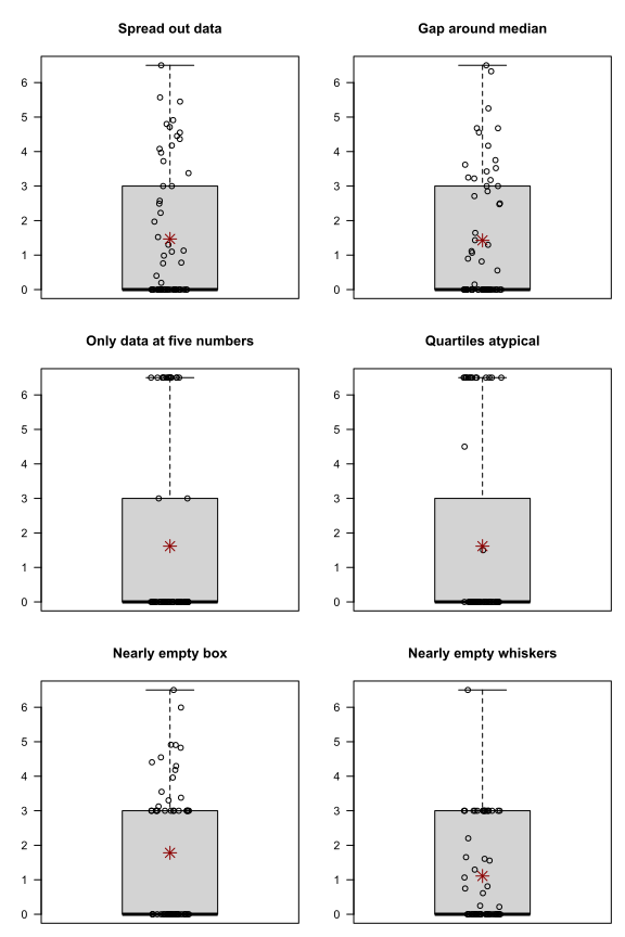
The situation is even worse in Figure 4: Now the median and the minimum coincide. In this case, there can’t be a gap around the median, and some values must correspond to the first hinge and the median.

draw_boxplots(five_numbers = c(0, 0, 0, 3, 6.5))

Figure 4: The median is also the minimum.

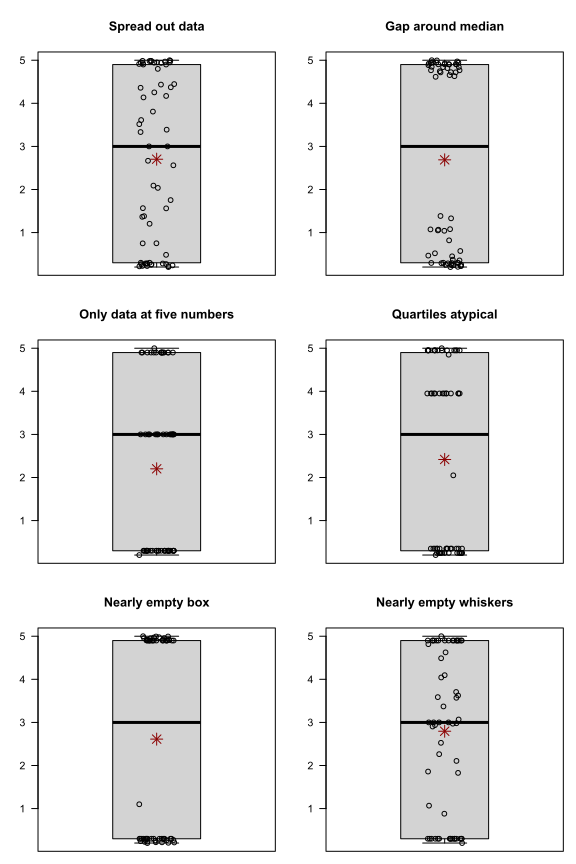
Figure 5 and Figure 6 highlight a counterintuitive aspect of boxplots: A larger box corresponds to a lower density in the middle 50% of the distribution, whereas a more compact box means that the middle 50% of the distribution is more tightly clustered around the median.

draw_boxplots(five_numbers = c(0.2, 0.3, 3, 4.9, 5))

Figure 5: A large box and tiny whiskers means that most data is concentrated near the extremes.

draw_boxplots(five_numbers = c(0.2, 2.1, 3, 3.5, 5))

Figure 6: And a compact box means that the data are more densely distributed in the middle 50% of the distribution.

The data underlying the boxplots can be inspected by setting the parameter show_data to TRUE.

Hopefully this convinces someone somewhere to add individual data points to their boxplots!

Software versions

devtools::session_info("attached")

─ Session info ───────────────────────────────────────────────────────────────
 setting  value
 version  R version 4.6.1 (2026-06-24 ucrt)
 os       Windows 11 x64 (build 26200)
 system   x86_64, mingw32
 ui       RTerm
 language (EN)
 collate  English_United Kingdom.utf8
 ctype    English_United Kingdom.utf8
 tz       Europe/Zurich
 date     2026-08-17
 pandoc   3.8.3 @ C:/Program Files/RStudio/resources/app/bin/quarto/bin/tools/ (via rmarkdown)
 quarto   1.9.38 @ C:\\Users\\VanhoveJ\\AppData\\Local\\Programs\\Quarto\\bin\\quarto.exe

──────────────────────────────────────────────────────────────────────────────

Footnotes

1. I ignore outliers in the remainder of this post.