Some tips on preparing your data for analysis

R
Author

Jan Vanhove

Published

June 18, 2015

How to prepare your spreadsheets so that they can be analysed efficiently is something you tend to learn on the job. In this blog post, I give some tips for organising datasets that I hope will be of use to students and researchers starting out in quantitative research.

Use self-explanatory names and labels, but keep them short

Try to minimise the need to consult the project codebook during the analysis. To this end, name your variables and their values sensibly. If you’re analysing questionnaire data, for instance, a variable name like Q3c means little to the analyst and requires them to refer back to the questionnaire or the codebook. Renaming this variable DialectUse makes it immediately clear that the variable likely encodes the degree to which the informant claims to use a dialect.

Similarly, a series of 0s and 1s in the Sex variable is uninformative. Sure, one of them will mean ‘man’ and the other ‘woman’, but which is which? Using the labels man and woman instead avoids any misunderstandings. Also note that values don’t have to be labelled numerically.

Lastly, use a consistent and unambiguous label to identify missing data. NA is usually a good choice, but don’t use 0 or -99 etc. Especially if you’re analysing numeric data, it may not be immediately obvious to the analyst that 0 or -99 don’t refer to actual measurements. (See exercises 2 and 3 on page 77 in my introduction to statistics, if you can read German.)

Transparent variables names and data labels facilitate the analysis because you don’t have to go back and forth between dataset and codebook to make sense of the data. A further benefit is that the code used for the analysis tends to be more readable, even months after the analysis has been conducted.

That said, when coming up with descriptive names and labels, try to keep them short. A variable name like HowOftenDoYouSpeakTheLocalDialectWithYourChild is self-explanatory but cumbersome to type repeatedly when analysing the data. DialectChild might be less self-explanatory but is easier to use.

Lastly, try to keep the following guidelines in mind:

  • Capitalisation matters. In R, an informant whose Sex is man is of a different gender than one whose Sex is Man. Any such confusions become clear soon enough when analysing the data and they’re pretty easy to take care of. But avoiding them is better for the analyst’s grumpiness level :)
  • Special characters are tricky. German Umlaut characters and French accents may show up without problems on your computer, but may require the manual specification of a character encoding on a different system. Try to either avoid special characters or know which character encoding you saved the dataset in (see the MS Office support page for Excel; LibreOffice users can just use the ‘Save as’ function and will be asked which encoding they prefer).
  • Don’t use spaces, question marks or exclamation marks in variable names.
  • Colour-coding is fine for your own use, but the colours get lost when the dataset is imported into a statistics program.
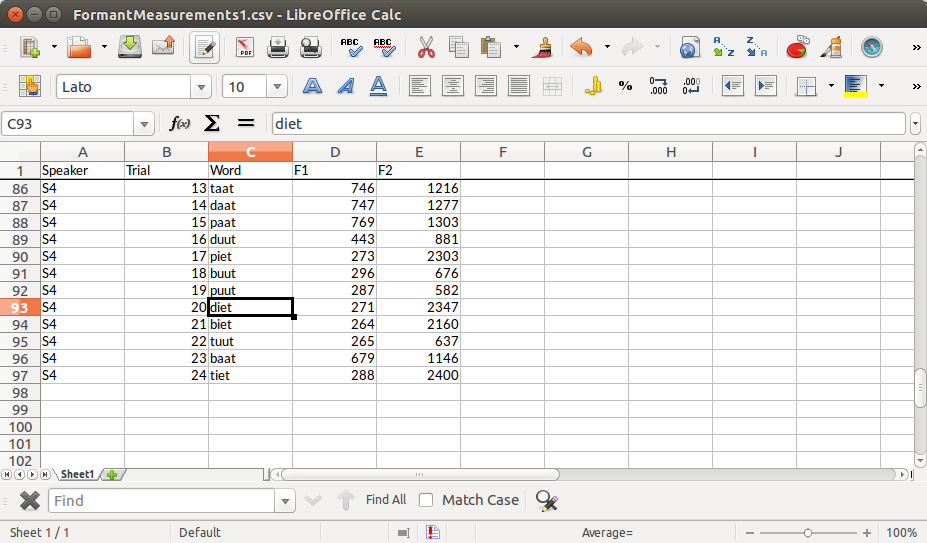
  • ‘Empty’ rows or columns may contain lingering spaces that mess up the dataset when it’s imported into a statistics program. By way of example, the csv file FormantMeasurements1.csv (available here) looks fine when it’s opened in a spreadsheet program:

    Example superfluous spaces

    When the dataset is imported into R, however, there seem to be two additional variables (X and X.1), some missing values (NA) and a Speaker without an ID:

    dat <- read.csv("http://janhove.github.io/downloads/FormantMeasurements1.csv",
                    stringsAsFactors = TRUE)
    summary(dat)
     Speaker     Trial            Word          F1               F2        
       : 2   Min.   : 1.00   baat   : 8   Min.   : 197.0   Min.   : 581.9  
     S1:24   1st Qu.: 6.75   biet   : 8   1st Qu.: 278.5   1st Qu.: 899.7  
     S2:24   Median :12.50   buut   : 8   Median : 350.2   Median :1544.8  
     S3:24   Mean   :12.50   daat   : 8   Mean   : 488.0   Mean   :1557.3  
     S4:24   3rd Qu.:18.25   diet   : 8   3rd Qu.: 772.2   3rd Qu.:2309.4  
             Max.   :24.00   duut   : 8   Max.   :1031.1   Max.   :2773.7  
             NA's   :2       (Other):50   NA's   :2        NA's   :2       
        X             X.1         
     Mode:logical   Mode:logical  
     NA's:98        NA's:98       


    The reason is that there are superfluous spaces in cells D99 and G9.
  • Similarly, a value label with a trailing space will be inconspicuous in your spreadsheet program but will affect how the dataset is read in into your statistics program. The csv file FormantMeasurements2.csv contains the same data as FormantMeasurements1.csv, but when read into R, there seem to be two Speakers with the same ID (S2):

    dat <- read.csv("http://janhove.github.io/downloads/FormantMeasurements2.csv",
                    stringsAsFactors = TRUE)
    summary(dat)
     Speaker      Trial            Word          F1               F2        
     S1 :24   Min.   : 1.00   baat   : 8   Min.   : 197.0   Min.   : 581.9  
     S2 :23   1st Qu.: 6.75   biet   : 8   1st Qu.: 278.5   1st Qu.: 899.7  
     S2 : 1   Median :12.50   buut   : 8   Median : 350.2   Median :1544.8  
     S3 :24   Mean   :12.50   daat   : 8   Mean   : 488.0   Mean   :1557.3  
     S4 :24   3rd Qu.:18.25   diet   : 8   3rd Qu.: 772.2   3rd Qu.:2309.4  
              Max.   :24.00   duut   : 8   Max.   :1031.1   Max.   :2773.7  
                              (Other):48                                    

    The reason is that there’s a trailing space in cell A28.

    Less obvious (because it doesn’t show up in the summary() output) is that there’s also a superfluous space in the Word column (the carrier word tiet occurs twice, once with and once without trailing space):

    levels(dat$Word)
     [1] "baat"  "biet"  "buut"  "daat"  "diet"  "duut"  "paat"  "piet"  "puut" 
    [10] "taat"  "tiet"  "tiet " "tuut" 

    As you can check for yourself, the trailing space is in cell C2.

    Problems like inconsistent capitalisation or trailing spaces are pretty easy to fix when you know they’re there, but they aren’t always obvious.

A ‘long’ data format is usually easier to manage than a ‘wide’ one

An example of a ‘wide’ dataset is Cognates_wide.csv (available here). The column Subject contains the participants’ IDs and every other column expresses whether the participant translated a given stimulus (e.g. ‘ägg’, ‘alltid’, ‘äta’ etc.) correctly. Every participant has their own row:

dat <- read.csv("http://janhove.github.io/downloads/Cognates_wide.csv",
                fileEncoding = "UTF-8",
                stringsAsFactors = TRUE)
head(dat)
  Subject agg alltid alska ata avskaffa bäbis bakgrund barn behärska bliva
1      64   0      0     1   1        0     0        1    0        0     0
2      78   0      0     0   0        0     0        1    0        0     0
3     134   0      0     0   0        0     0        1    0        0     0
4     230   0      0     0   0        0     0        1    0        0     0
5     288   0      0     0   0        0     0        1    0        0     0
6     326   0      0     0   0        0     1        1    1        0     0
  blomma borgmästare borja branna butelj byrå choklad cyckel egenskap elev
1      1           0     0      1      0    0       0      0        0    0
2      1           0     0      1      0    0       0      1        0    0
3      1           0     0      1      0    0       0      0        0    0
4      0           1     0      1      0    0       0      0        0    0
5      0           0     0      1      0    0       0      0        0    0
6      1           0     0      1      0    0       0      1        0    1
  ensam fåtölj fiende flicka fonster försiktig forsoka forst forsvinna
1     0      0      1      0       1         1       0     0         1
2     0      0      0      0       1         1       0     0         1
3     1      0      0      0       1         0       0     0         1
4     0      0      1      0       1         1       0     0         1
5     0      0      0      0       1         1       0     0         0
6     0      0      1      0       1         1       0     0         1
  förutsättning fotboll fraga frasch full ga grupp hård häst hemlig ingenjor
1             1       1     1      1    1  1     0    1    0      0        1
2             0       1     1      1    1  1     0    1    0      0        1
3             0       1     0      1    0  0     1    0    0      1        1
4             0       1     1      0    1  0     0    1    0      0        1
5             0       1     0      0    0  0     0    1    0      0        1
6             0       1     0      1    1  0     0    1    0      0        1
  intryck is kagel kanel karnkraftverk kejsar kniv konst korruption kung kyrka
1       0  0     0     0             0      0    1     1          0    0     1
2       0  0     0     0             1      0    1     1          0    0     1
3       0  0     0     0             1      0    1     1          0    0     0
4       0  0     0     0             0      1    1     1          0    0     1
5       0  0     0     0             1      0    0     1          0    0     0
6       0  0     0     0             1      1    0     1          0    0     1
  kyssa lang larm leka löpa markvardig mjölk möjlig mycket nackdel öppna ost
1     1    1    1    0    0          1     0      0      0       0     1   1
2     1    1    0    0    0          0     1      0      0       0     1   1
3     0    0    1    0    0          1     1      0      0       1     1   1
4     1    1    0    0    0          0     1      1      0       0     1   1
5     0    0    1    0    0          1     0      0      0       0     0   0
6     1    1    0    0    0          1     1      0      0       0     0   1
  overraska översätta paraply passiv potatis rådhus rytmisk saliv sitta
1         0         0       1      1       1      1       1     1     1
2         0         0       1      1       1      1       1     0     1
3         0         1       1      1       1      1       1     0     1
4         0         0       1      0       0      1       1     0     1
5         0         0       0      1       0      0       0     0     0
6         0         0       0      1       1      1       1     0     1
  sjalvstandig skarm skola skön skriva skrubba skyskrapa smart smink söka
1            1     0     1    1      0       1         1     1     0    0
2            0     0     1    0      0       0         0     0     1    0
3            1     0     0    0      0       0         1     0     1    0
4            0     0     1    0      0       0         1     1     0    1
5            1     0     0    0      0       0         1     1     0    0
6            0     0     1    1      0       0         0     1     1    0
  spegel språk städa stjärn sverige tanka tårta torsdag trakig tunga tvivla
1      1     1     0      0       0     1     1       1      0     0      1
2      1     1     0      1       0     0     1       0      0     0      0
3      0     0     0      1       0     1     0       1      0     0      0
4      1     1     0      1       0     0     1       1      0     0      0
5      1     0     0      1       0     0     0       1      0     0      0
6      1     1     0      1       0     1     1       1      0     1      0
  tydlig ursprung värld varm vaxla viktig ytterst
1      0        1     0    1     1      1       0
2      0        1     0    1     1      1       0
3      0        1     0    1     1      0       0
4      0        1     0    1     0      1       0
5      0        0     0    1     1      1       0
6      0        1     0    1     1      1       0

In a ‘long’ dataset (e.g. Cognates_long.csv), the data are arranged differently, typically with one row per ‘observation unit’:

dat <- read.csv("http://janhove.github.io/downloads/Cognates_long.csv",
                fileEncoding = "UTF-8", stringsAsFactors = TRUE)
head(dat); tail(dat)
  Subject Stimulus Correct
1    1034      agg       0
2    2151      agg       0
3    9022      agg       0
4    7337      agg       0
5    8477      agg       0
6    6544      agg       0
      Subject Stimulus Correct
16295    5290  ytterst       0
16296    3125  ytterst       0
16297    4137  ytterst       0
16298    1967  ytterst       0
16299    8942  ytterst       0
16300    9913  ytterst       0

I prefer long datasets for the following reasons:

  • The statistical tools I usually work with (mixed-effects models) require data in a long format.

  • It’s easier to add information to a long than to a wide dataset. For instance, if I wanted to add the order in which the participants saw the stimuli to the wide format, I’d have to add 100 columns to save the trial numbers (i.e. aggTrial, alltidTrial etc.). I’d only have to add one column (Trial) in the case of long data.

  • While wide datasets are useful for analytical techniques such as principal component analysis, factor analysis or structural equation modeling as well as paired t-tests, I find it easier to convert a long dataset to a wide dataset than vice versa, especially if the dataset contains additional information about the stimuli or trials.

A useful package for converting long data to wide data and vice versa is reshape2, whose use is helpfully explained by Sean Anderson.

Managing several smallish datasets and then joining them before the analysis is easier than handling one large dataset

Complex datasets often contain repeated data. For instance, we could add the participants’ age to Cognates_long.csv above, but we’d have to repeat each participant’s age 100 times. Similarly, we could add information about the stimuli to Cognates_long.csv (e.g. their length in phonemes), but we’d have to repeat each stimulus’s length 163 times (once for each participant). In such cases, I find it easiest to compile several smaller datasets with as little information repeated as possible and to combine them when needed. That way, if I make a mistake when entering the data, I’ll only have to correct it once and then recombine the datasets.

Here’s an illustration of what I mean. The participants’ accuracy per stimulus is stored in Cognates_long.csv.

dat <- read.csv("http://janhove.github.io/downloads/Cognates_long.csv",
                fileEncoding = "UTF-8", stringsAsFactors = TRUE)

Background information about the participants is available in ParticipantInformation.csv:

participants <- read.csv("http://janhove.github.io/downloads/ParticipantInformation.csv",
                         fileEncoding = "UTF-8", stringsAsFactors = TRUE)
summary(participants)
    Subject         Sex          Age            NrLang         DS.Span     
 Min.   :  64   female:90   Min.   :10.00   Min.   :1.000   Min.   :2.000  
 1st Qu.:2990   male  :73   1st Qu.:16.00   1st Qu.:2.000   1st Qu.:4.000  
 Median :5731               Median :39.00   Median :3.000   Median :4.000  
 Mean   :5317               Mean   :40.28   Mean   :3.067   Mean   :4.613  
 3rd Qu.:7769               3rd Qu.:59.50   3rd Qu.:4.000   3rd Qu.:5.000  
 Max.   :9913               Max.   :86.00   Max.   :9.000   Max.   :8.000  
                                                                           
    DS.Total          GmVoc           Raven       EnglishScore  
 Min.   : 2.000   Min.   : 4.00   Min.   : 0.0   Min.   : 3.00  
 1st Qu.: 5.000   1st Qu.:29.00   1st Qu.:12.0   1st Qu.:20.75  
 Median : 6.000   Median :34.00   Median :19.0   Median :31.00  
 Mean   : 6.374   Mean   :30.24   Mean   :17.8   Mean   :28.30  
 3rd Qu.: 7.500   3rd Qu.:36.00   3rd Qu.:24.0   3rd Qu.:37.00  
 Max.   :12.000   Max.   :41.00   Max.   :35.0   Max.   :44.00  
                  NA's   :1                      NA's   :3      

The entries in the Subject column in Cognates_long.csv correspond to those in the same column in ParticipantInformation.csv. Using merge(), we can add the information in the latter dataset to the corresponding rows in the former:

dat <- merge(dat, participants, "Subject")
head(dat); tail(dat)
  Subject      Stimulus Correct    Sex Age NrLang DS.Span DS.Total GmVoc Raven
1      64         forst       0 female  27      4       6        7    34    28
2      64          löpa       0 female  27      4       6        7    34    28
3      64           ost       1 female  27      4       6        7    34    28
4      64         tunga       0 female  27      4       6        7    34    28
5      64 förutsättning       1 female  27      4       6        7    34    28
6      64         ensam       0 female  27      4       6        7    34    28
  EnglishScore
1           42
2           42
3           42
4           42
5           42
6           42
      Subject  Stimulus Correct    Sex Age NrLang DS.Span DS.Total GmVoc Raven
16295    9913     grupp       1 female  40      3       5        8    29    17
16296    9913      kung       0 female  40      3       5        8    29    17
16297    9913     städa       0 female  40      3       5        8    29    17
16298    9913     tanka       1 female  40      3       5        8    29    17
16299    9913 skyskrapa       0 female  40      3       5        8    29    17
16300    9913   rytmisk       0 female  40      3       5        8    29    17
      EnglishScore
16295           17
16296           17
16297           17
16298           17
16299           17
16300           17

Similarly, we can add information about the stimuli, available in StimulusInformation.csv, to dat.

stimuli <- read.csv("http://janhove.github.io/downloads/StimulusInformation.csv",
                    fileEncoding = "UTF-8", stringsAsFactors = TRUE)
summary(stimuli)
     Stimulus      Status      Duration          Swedish          German  
 agg     : 1   profile:10   Min.   : 516.0   2st     : 1   abschaffen: 1  
 alltid  : 1   target :90   1st Qu.: 708.8   2v@raska: 1   ai        : 1  
 alska   : 1                Median : 869.5   alltid  : 1   aig@nSaft : 1  
 ata     : 1                Mean   : 843.4   avskaffa: 1   aindruk   : 1  
 avskaffa: 1                3rd Qu.: 929.8   b2rja   : 1   ainzam    : 1  
 bäbis   : 1                Max.   :1264.0   babis   : 1   (Other)   :75  
 (Other) :94                NA's   :50       (Other) :94   NA's      :20  
       English        French       LevGer           LevEng      
 @larm     : 1   alarm   : 1   Min.   :0.1429   Min.   :0.0000  
 ais       : 1   bebe    : 1   1st Qu.:0.4000   1st Qu.:0.4000  
 b2rn      : 1   bureau  : 1   Median :0.5000   Median :1.0000  
 baby      : 1   butEj   : 1   Mean   :0.5859   Mean   :0.6997  
 background: 1   cannelle: 1   3rd Qu.:0.8333   3rd Qu.:1.0000  
 (Other)   :42   (Other) :18   Max.   :1.0000   Max.   :1.0000  
 NA's      :53   NA's    :77                                    
     LevFre         FreqGerman        FreqEnglish       FreqFrench   
 Min.   :0.0000   Min.   :   0.000   Min.   :   0.0   Min.   :    0  
 1st Qu.:1.0000   1st Qu.:   0.932   1st Qu.:   0.0   1st Qu.:    0  
 Median :1.0000   Median :  20.020   Median :   0.0   Median :    0  
 Mean   :0.8529   Mean   : 109.714   Mean   : 119.4   Mean   :  237  
 3rd Qu.:1.0000   3rd Qu.:  60.138   3rd Qu.:  43.6   3rd Qu.:    0  
 Max.   :1.0000   Max.   :3460.090   Max.   :3793.0   Max.   :22823  
                                                                     

The shared denominator of both datasets is stored in the column Stimulus:

dat <- merge(dat, stimuli, "Stimulus")
head(dat); tail(dat)
  Stimulus Subject Correct    Sex Age NrLang DS.Span DS.Total GmVoc Raven
1      agg    7479       0   male  25      4       8       11    38    34
2      agg    7337       0 female  49      3       4        5    36    19
3      agg    2846       0 female  11      3       4        6     4    15
4      agg    5153       0 female  51      3       4        6    37    18
5      agg    6510       0 female  41      2       5        8    34    30
6      agg    6329       0 female  56      3       5        6    37    21
  EnglishScore Status Duration Swedish German English French LevGer LevEng
1           43 target      547      Eg     ai      Eg   <NA>      1      0
2           30 target      547      Eg     ai      Eg   <NA>      1      0
3            6 target      547      Eg     ai      Eg   <NA>      1      0
4           37 target      547      Eg     ai      Eg   <NA>      1      0
5           40 target      547      Eg     ai      Eg   <NA>      1      0
6           42 target      547      Eg     ai      Eg   <NA>      1      0
  LevFre FreqGerman FreqEnglish FreqFrench
1      1      24.06       26.04          0
2      1      24.06       26.04          0
3      1      24.06       26.04          0
4      1      24.06       26.04          0
5      1      24.06       26.04          0
6      1      24.06       26.04          0
      Stimulus Subject Correct    Sex Age NrLang DS.Span DS.Total GmVoc Raven
16295  ytterst    1350       0   male  43      4       7       10    38    31
16296  ytterst    7337       0 female  49      3       4        5    36    19
16297  ytterst    8578       0   male  11      2       4        6     9    20
16298  ytterst     717       0 female  15      2       5        6    29    21
16299  ytterst    8805       0   male  70      4       4        4    35    22
16300  ytterst    9912       0   male  10      2       4        4     9    14
      EnglishScore Status Duration Swedish   German English French LevGer
16295           38 target       NA ytterst ausserst    <NA>   <NA>    0.5
16296           30 target       NA ytterst ausserst    <NA>   <NA>    0.5
16297           17 target       NA ytterst ausserst    <NA>   <NA>    0.5
16298           25 target       NA ytterst ausserst    <NA>   <NA>    0.5
16299           35 target       NA ytterst ausserst    <NA>   <NA>    0.5
16300            9 target       NA ytterst ausserst    <NA>   <NA>    0.5
      LevEng LevFre FreqGerman FreqEnglish FreqFrench
16295      1      1      23.19           0          0
16296      1      1      23.19           0          0
16297      1      1      23.19           0          0
16298      1      1      23.19           0          0
16299      1      1      23.19           0          0
16300      1      1      23.19           0          0

Reading tip

Hadley Wickham’s Tidy data, while primarily geared towards software developers, is well worth a read.

Software versions

devtools::session_info()
─ Session info ───────────────────────────────────────────────────────────────
 setting  value
 version  R version 4.3.1 (2023-06-16)
 os       Ubuntu 22.04.3 LTS
 system   x86_64, linux-gnu
 ui       X11
 language en_US
 collate  en_US.UTF-8
 ctype    en_US.UTF-8
 tz       Europe/Zurich
 date     2023-08-26
 pandoc   3.1.1 @ /usr/lib/rstudio/resources/app/bin/quarto/bin/tools/ (via rmarkdown)

─ Packages ───────────────────────────────────────────────────────────────────
 package     * version date (UTC) lib source
 cachem        1.0.6   2021-08-19 [2] CRAN (R 4.2.0)
 callr         3.7.3   2022-11-02 [1] CRAN (R 4.3.1)
 cli           3.6.1   2023-03-23 [1] CRAN (R 4.3.0)
 crayon        1.5.2   2022-09-29 [1] CRAN (R 4.3.1)
 devtools      2.4.5   2022-10-11 [1] CRAN (R 4.3.1)
 digest        0.6.29  2021-12-01 [2] CRAN (R 4.2.0)
 ellipsis      0.3.2   2021-04-29 [2] CRAN (R 4.2.0)
 evaluate      0.15    2022-02-18 [2] CRAN (R 4.2.0)
 fastmap       1.1.0   2021-01-25 [2] CRAN (R 4.2.0)
 fs            1.5.2   2021-12-08 [2] CRAN (R 4.2.0)
 glue          1.6.2   2022-02-24 [2] CRAN (R 4.2.0)
 htmltools     0.5.5   2023-03-23 [1] CRAN (R 4.3.0)
 htmlwidgets   1.6.2   2023-03-17 [1] CRAN (R 4.3.1)
 httpuv        1.6.11  2023-05-11 [1] CRAN (R 4.3.1)
 jsonlite      1.8.7   2023-06-29 [1] CRAN (R 4.3.1)
 knitr         1.39    2022-04-26 [2] CRAN (R 4.2.0)
 later         1.3.1   2023-05-02 [1] CRAN (R 4.3.1)
 lifecycle     1.0.3   2022-10-07 [1] CRAN (R 4.3.0)
 magrittr      2.0.3   2022-03-30 [1] CRAN (R 4.3.0)
 memoise       2.0.1   2021-11-26 [2] CRAN (R 4.2.0)
 mime          0.10    2021-02-13 [2] CRAN (R 4.0.2)
 miniUI        0.1.1.1 2018-05-18 [1] CRAN (R 4.3.1)
 pkgbuild      1.4.2   2023-06-26 [1] CRAN (R 4.3.1)
 pkgload       1.3.2.1 2023-07-08 [1] CRAN (R 4.3.1)
 prettyunits   1.1.1   2020-01-24 [2] CRAN (R 4.2.0)
 processx      3.8.2   2023-06-30 [1] CRAN (R 4.3.1)
 profvis       0.3.8   2023-05-02 [1] CRAN (R 4.3.1)
 promises      1.2.0.1 2021-02-11 [1] CRAN (R 4.3.1)
 ps            1.7.5   2023-04-18 [1] CRAN (R 4.3.1)
 purrr         1.0.1   2023-01-10 [1] CRAN (R 4.3.0)
 R6            2.5.1   2021-08-19 [2] CRAN (R 4.2.0)
 Rcpp          1.0.11  2023-07-06 [1] CRAN (R 4.3.1)
 remotes       2.4.2   2021-11-30 [2] CRAN (R 4.2.0)
 rlang         1.1.1   2023-04-28 [1] CRAN (R 4.3.0)
 rmarkdown     2.21    2023-03-26 [1] CRAN (R 4.3.0)
 rstudioapi    0.14    2022-08-22 [1] CRAN (R 4.3.0)
 sessioninfo   1.2.2   2021-12-06 [2] CRAN (R 4.2.0)
 shiny         1.7.4.1 2023-07-06 [1] CRAN (R 4.3.1)
 stringi       1.7.12  2023-01-11 [1] CRAN (R 4.3.1)
 stringr       1.5.0   2022-12-02 [1] CRAN (R 4.3.0)
 urlchecker    1.0.1   2021-11-30 [1] CRAN (R 4.3.1)
 usethis       2.2.2   2023-07-06 [1] CRAN (R 4.3.1)
 vctrs         0.6.3   2023-06-14 [1] CRAN (R 4.3.0)
 xfun          0.39    2023-04-20 [1] CRAN (R 4.3.0)
 xtable        1.8-4   2019-04-21 [1] CRAN (R 4.3.1)
 yaml          2.3.5   2022-02-21 [2] CRAN (R 4.2.0)

 [1] /home/jan/R/x86_64-pc-linux-gnu-library/4.3
 [2] /usr/local/lib/R/site-library
 [3] /usr/lib/R/site-library
 [4] /usr/lib/R/library

──────────────────────────────────────────────────────────────────────────────