Author: Jan Vanhove (@, www)
Last update: 12 September 2018
Introduction
The accompanying article can be downloaded from
PsyArxiv.
Before we begin
I'll assume you have some basic knowledge of R
(R Core Team, 2018),
such as how you can read in CSV files.
In addition, if you haven't already, install and load the tidyverse suite
(Wickham, 2017):
install.packages("tidyverse")
## ---- Attaching packages -------------------------------------------------------------------- tidyverse 1.2.1 ----
## V ggplot2 2.2.1     V purrr   0.2.4
## V tibble  1.4.2     V dplyr   0.7.4
## V tidyr   0.8.0     V stringr 1.2.0
## V readr   1.1.1     V forcats 0.2.0
## ---- Conflicts ------------------------------------------------------------------------- tidyverse_conflicts() ----
## X dplyr::filter() masks stats::filter()
## X dplyr::lag()    masks stats::lag()
# install the devtools package if needed:
# install.packages("devtools")
library(devtools)
install_github("janhove/cannonball")
# Set random seed
set.seed(42)
# Change default plotting theme (just my preference)
theme_set(theme_bw(10))
Example 1: A simple linear regression model
Download the data for DeKeyser et al.'s (2010) Israel study
from my website
to your R working directory. (Use "save link as" for this;
don't open the file in Excel and then save it.
Excel has a way of messing up CSV files.)
Then read it in and refit Vanhove's (2013) linear model:
# Read in data
d <- read.csv("dekeyser2010.csv")

# Fit linear model
m <- lm(GJT ~ AOA, data = d)
summary(m)
##
## Call:
## lm(formula = GJT ~ AOA, data = d)
##
## Residuals:
##     Min      1Q  Median      3Q     Max
## -55.380  -7.338   2.662   9.777  36.204
##
## Coefficients:
##             Estimate Std. Error t value Pr(>|t|)
## (Intercept) 187.1297     4.2762   43.76  < 2e-16 ***
## AOA          -1.2292     0.1226  -10.02 1.96e-14 ***
## ---
## Signif. codes:  0 '***' 0.001 '**' 0.01 '*' 0.05 '.' 0.1 ' ' 1
##
## Residual standard error: 16.23 on 60 degrees of freedom
## Multiple R-squared:  0.626,	Adjusted R-squared:  0.6198
## F-statistic: 100.4 on 1 and 60 DF,  p-value: 1.965e-14
Linearity
The function for generating a line-up of 19 simulated datasets
alongside the real dataset is parade(). You need
to supply to it the name of a fitted model; in this case m.
# Generate the parade and store it to a separate object
my_parade <- parade(m)
By default, parade() generates a tibble
(the tidyverse version of a data frame) with the model's
predictor and outcome variables as well as its fitted
values and residuals (and transformations thereof):
## # A tibble: 6 x 7
##     AOA   GJT .fitted .resid .abs_resid .sqrt_abs_resid .sample
##   <int> <dbl>   <dbl>  <dbl>      <dbl>           <dbl>   <int>
## 1     4   204     186  18.9       18.9             4.35       1
## 2     5   172     184 -12.3       12.3             3.51       1
## 3     6   186     183   2.86       2.86            1.69       1
## 4     6   190     183   7.24       7.24            2.69       1
## 5     7   185     181   3.67       3.67            1.92       1
## 6     7   177     181 - 4.62       4.62            2.15       1
If your dataset contains variables that weren't part
of the model and you wish to include these in the line-up,
supply your dataset as the input to the optional full_data
parameter:
# my_parade <- parade(m, full_data = d)
Currently, parade() accepts models fitted with lm()
as well as models fitted with the gam() function
from the mgcv package (Wood, 2018).
If there's sufficient demand (i.e., once I need it myself),
other models may follow.
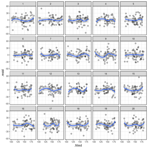
To check for residual patterns due to unmodelled nonlinearities,
you can plot the residual values (.resid) against the fitted values
(.fitted). The ggplot() call for this is:
ggplot(my_parade,         # name of the parade object
       aes(x = .fitted,   # fitted values on x-axis
           y = .resid)) + # residual values on y-axis
  geom_point(shape = 1) + # plot them as hollow points
  geom_smooth() +         # add a nonlinear scatterplot smoother
  facet_wrap(~ .sample)
## `geom_smooth()` using method = 'loess'
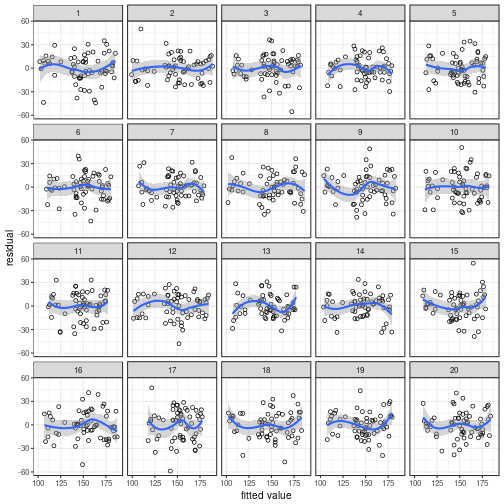
A quicker way to draw the same plot is to use
cannonball's lin_plot() function:
## `geom_smooth()` using method = 'loess'
Once you've made your mind up about which plot evinces
the strongest pattern, reveal the true data's position
using reveal():
## The true data are in position 3.
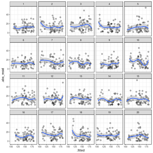
Constant variance
# Generate a new parade
my_parade <- parade(m)
ggplot(my_parade,
       aes(x = .fitted,
           y = .abs_resid)) + # use .sqrt_abs_resid if you prefer
                              # to plot the square roots of the
                              # residuals' absolute values
  geom_point(shape = 1) +
  geom_smooth() +
  facet_wrap(~ .sample)
## `geom_smooth()` using method = 'loess'
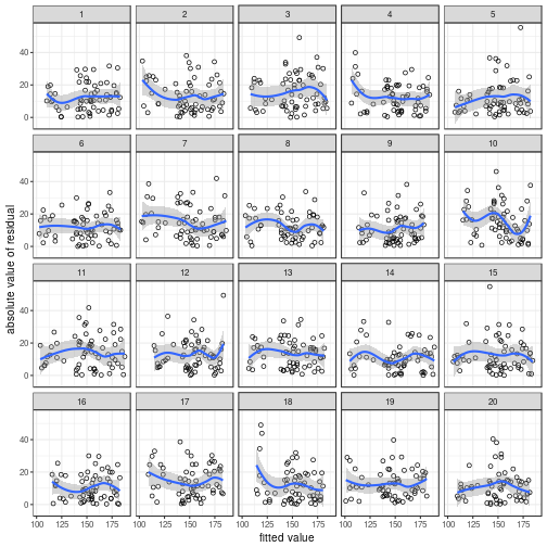
You can also use the var_plot() function
if you don't want to tinker with these graphs.
## `geom_smooth()` using method = 'loess'
## The true data are in position 5.
Take Five is the instantly recognisable
jazz hit penned by Paul Desmond.
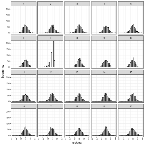
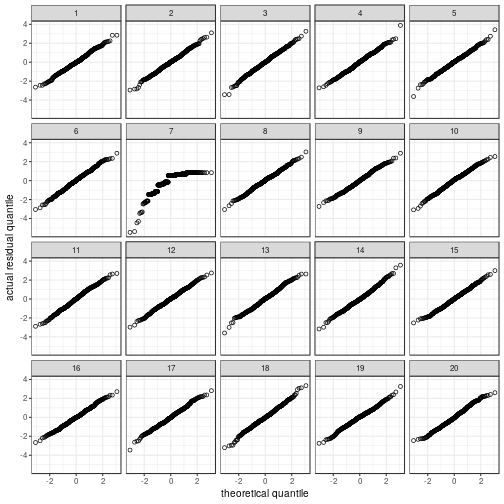
Normality
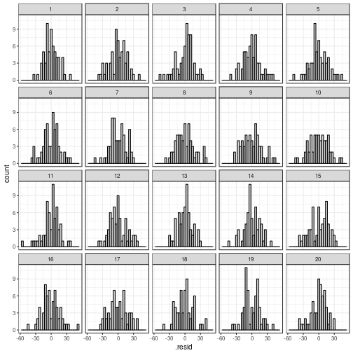
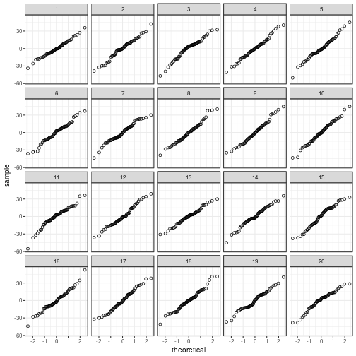
Depending on what you find easiest to read, you
can plot the residuals in a histogram or in a
quantile–quantile plot.
# New line-up
my_parade <- parade(m)

# Histogram
ggplot(my_parade,
       aes(x = .resid)) +
  geom_histogram(bins = 30, # you can change this if you want
                 fill = "lightgrey", colour = "black") +
  facet_wrap(~ .sample)
# Quantile-quantile plot
ggplot(my_parade,
       aes(sample = .resid)) +
  stat_qq(shape = 1) +
  facet_wrap(~ .sample)
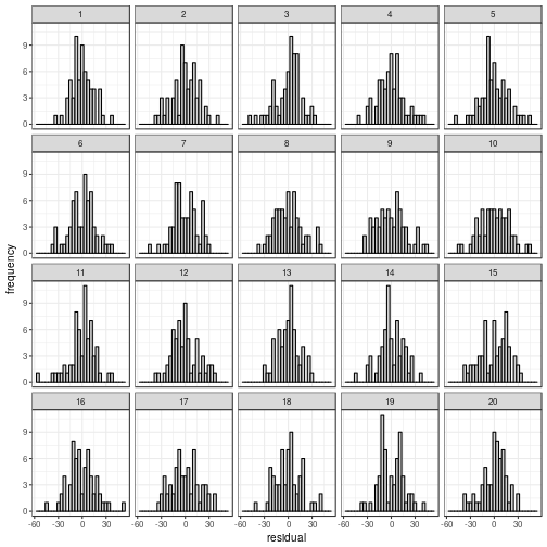
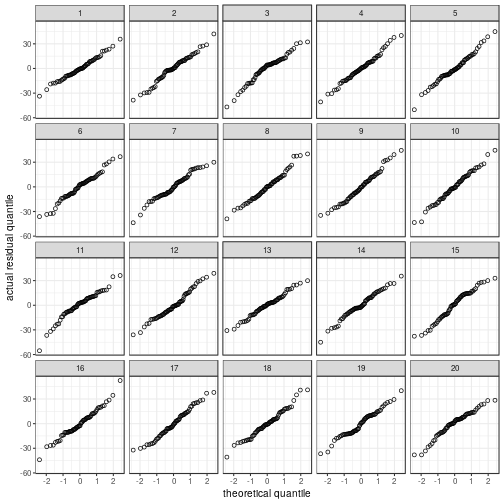
Short-hand functions to draw these graphs are:
## The true data are in position 11.
Impossible data
This is similar to what is known
as posterior predictive checking in Bayesian statistics.
The idea is that you check if the model occasionally
generates data that are simply impossible given what you
know about the subject-matter. Here I draw 19 additional
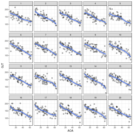
scatterplots of the (simulated) AOA–GJT relationship.
# New line-up
my_parade <- parade(m)
ggplot(my_parade,
       aes(x = AOA,
           y = GJT)) +
  geom_point(shape = 1) +
  geom_smooth() +
  facet_wrap(~ .sample)
## `geom_smooth()` using method = 'loess'
The model sometimes generates GJT data
outside of the possible range (0 to 204),
showing that we know something about these
data that the model doesn't. In principle,
we could embed this knowledge in a more
complex model, but doing so is beyond the scope
of this tutorial.
Example 2: ANOVA on Likert-scale data
I cleaned up Lee et al.'s (2018) data set
so that it's easier to read it into R. With
their consent, I've put it on my website
from where you can download it to your working directory.
(Use "save link as"; don't open it in Excel and then save it.)
Then read in the dataset:
# Read in data
d <- read.csv("lee2018_s2.csv")
Refitting ANOVAs and t-tests as linear models
If you analysed your data using a Student's t-test
and you want to use the parade() function,
you need to refit the test as a linear model.
This is pretty easy. Let's say your outcome variable
is creatively named Y, your predictor (group) variable
is called X and both are in a dataset called my_data.
To run the t-test, you'd use this command:
# generic example
t.test(Y ~ X, data = my_data, var.equal = TRUE)
You will obtain the same results if you use the lm()
function instead:
# generic example
my_model <- lm(Y ~ X, data = my_data)
summary(my_model)
Similarly, an ANOVA or ANCOVA can be reproduced as a linear model.
If you have more than one predictor, just add the different predictors
to the model using '+'. If your ANOVA contains an interaction,
use '*' between the interacting predictors:
# Fit linear model
m <- lm(Happiness ~ PurchaseType * SocialClass, data = d)
summary(m)
##
## Call:
## lm(formula = Happiness ~ PurchaseType * SocialClass, data = d)
##
## Residuals:
##     Min      1Q  Median      3Q     Max
## -5.4671 -0.3793  0.5329  0.6207  0.8385
##
## Coefficients:
##                                     Estimate Std. Error t value Pr(>|t|)
## (Intercept)                          6.16154    0.08492  72.556  < 2e-16
## PurchaseTypematerial                 0.21777    0.12367   1.761  0.07890
## SocialClasslow                       0.30557    0.11567   2.642  0.00853
## PurchaseTypematerial:SocialClasslow -0.37502    0.18619  -2.014  0.04456
##
## (Intercept)                         ***
## PurchaseTypematerial                .
## SocialClasslow                      **
## PurchaseTypematerial:SocialClasslow *
## ---
## Signif. codes:  0 '***' 0.001 '**' 0.01 '*' 0.05 '.' 0.1 ' ' 1
##
## Residual standard error: 0.9682 on 465 degrees of freedom
## Multiple R-squared:  0.01544,	Adjusted R-squared:  0.009085
## F-statistic:  2.43 on 3 and 465 DF,  p-value: 0.06457
Constant variance
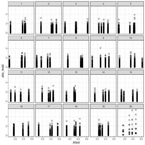
If we check for constant variance in the same
way as before, it's ridiculously easy to spot
the actual data plot:
my_parade <- parade(m)
ggplot(my_parade,
       aes(x = .fitted,
           y = .abs_resid)) +
  geom_point(shape = 1) +
  # geom_smooth() + # uncomment this line if you like warnings
  facet_wrap(~ .sample)
As discussed in the accompanying paper,
I suggest to instead compute the variance or
standard deviation of the residuals per cell,
so that we don't confuse one clear deficiency of the model
(not taking into account the categorical nature of the outcome)
with another possible one (heteroskedasticity).
The parade_summary() function makes it easier
to compute measures. It takes as its input
an object generated by the parade() function:
my_parade <- parade(m)
my_parade_summary <- parade_summary(my_parade)
For each cell, parade_summary() computes the
mean residual (.mean_resid),
the mean absolute residual (.mean_abs_resid),
the mean of the square roots of the absolute residuals (.mean_sqrt_abs_resid),
the standard deviation of the residuals (.sd),
the variance of the residuals (.var),
and the cell size (.n).
It also labels each unique combination of non-outcome
variables (.cell).
The mean residual per cell may be useful to check if there
are any interaction patterns or predictors that still need
to be accounted for; the other measures are
useful for checking for non-constant variance.
## # A tibble: 6 x 11
##   .sample PurchaseType SocialClass .fitted     .mean_resid .mean_abs_resid
##     <int> <fct>        <fct>         <dbl>           <dbl>           <dbl>
## 1       1 experiential high           6.09        2.99e-16           0.850
## 2       1 experiential low            6.48       -1.45e-17           0.771
## 3       1 material     high           6.31       -5.65e-17           0.913
## 4       1 material     low            6.37       -3.74e-16           0.808
## 5       2 experiential high           6.12       -6.33e-16           0.799
## 6       2 experiential low            6.39        7.47e-16           0.769
## # ... with 5 more variables: .mean_sqrt_abs_resid <dbl>, .var <dbl>,
## #   .sd <dbl>, .n <int>, .cell <fct>
By default, the cells are defined as the unique
combinations of all non-outcome variable values
present in the parade object, even those that
weren't used for fitting the model.
If you only want to define the cells using
the predictors actually used in the model,
specify the predictors_only parameter appropriately:
# my_parade_summary <- parade_summary(my_parade, predictors_only = TRUE)
Incidentally, parade_summary() will throw
a bunch of warnings if it's used in cases where I
don't think that doing so is too useful (e.g.,
fairly continuous outcome data, non-categorical
predictors, small cell sizes).
The output of parade_summary()
can also be plotted using ggplot():
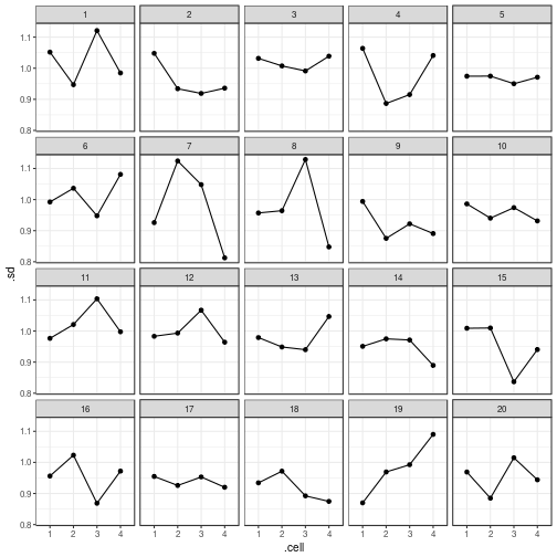
ggplot(my_parade_summary,
       aes(x = .cell,
           y = .sd,
           group = 1)) +
  geom_point() +
  geom_line() +
  facet_wrap(~ .sample)
You can also use the var_plot() function to draw
this plot:
var_plot(my_parade_summary)
reveal(my_parade_summary)
## The true data are in position 19.
Hey Nineteen is one of my favourite Steely Dan tracks.
Normality
Regardless of whether the residuals
are displayed in a histogram or in a
QQ plot, the actual data panel sticks out.
my_parade <- parade(m)
norm_hist(my_parade)
If the amount of data doesn't fully reassure
you, you can construct the confidence intervals
using a nonparametric bootstrap. The confidence
intervals are pretty much the same as those
constructed using t-distributions, which
technically require normality. That said,
it may be a good idea to fit these
data in an ordinal regression model
(done but not shown here; Lee et al.'s (2018)
substantive conclusions don't change).
# Check results with bootstrap -----

# Empty matrix that'll contain the bootstrap
# estimates for the model's 4 coefficients.
bs_est <- matrix(ncol = length(coef(m)), nrow = 20000)

for (i in 1:20000) {
  # Draw bootstrap sample. Keep cell sizes intact.
  d_bs <- d %>%
    group_by(PurchaseType, SocialClass) %>%
    sample_frac(1, replace = TRUE) %>%
    ungroup()
  # Refit model on bootstrap sample
  m_bs <- lm(Happiness ~ PurchaseType * SocialClass, data = d_bs)
  # Extract coefficient estimates
  bs_est[i, ] <- coef(m_bs)
}

# The t-distribution based 95% confidence intervals:
confint(m)
##                                           2.5 %       97.5 %
## (Intercept)                          5.99466261  6.328414314
## PurchaseTypematerial                -0.02524254  0.460786310
## SocialClasslow                       0.07826846  0.532865138
## PurchaseTypematerial:SocialClasslow -0.74088883 -0.009147157
# The bootstrap-based 95% confidence intervals (percentile method)
t(apply(bs_est, 2, quantile, probs = c(0.025, 0.975)))
##             2.5%       97.5%
## [1,]  6.00769231 6.307692308
## [2,] -0.02016578 0.447751989
## [3,]  0.08704200 0.517634109
## [4,] -0.75181717 0.001893036
Software versions
devtools::session_info(c("tidyverse", "cannonball"))
## Session info -------------------------------------------------------------
##  setting  value
##  version  R version 3.4.4 (2018-03-15)
##  system   x86_64, linux-gnu
##  ui       X11
##  language (EN)
##  collate  en_US.UTF-8
##  tz       Europe/Brussels
##  date     2018-09-12
## Packages -----------------------------------------------------------------
##  package      * version    date       source
##  assertthat     0.2.0      2017-04-11 CRAN (R 3.4.2)
##  backports      1.1.2      2017-12-13 CRAN (R 3.4.2)
##  base64enc      0.1-3      2015-07-28 CRAN (R 3.4.2)
##  BH             1.66.0-1   2018-02-13 CRAN (R 3.4.2)
##  bindr          0.1        2016-11-13 CRAN (R 3.4.2)
##  bindrcpp     * 0.2        2017-06-17 CRAN (R 3.4.2)
##  broom          0.4.3      2017-11-20 CRAN (R 3.4.2)
##  callr          2.0.2      2018-02-11 CRAN (R 3.4.2)
##  cannonball   * 0.0.0.9000 2018-09-11 Github (janhove/cannonball@197304f)
##  cellranger     1.1.0      2016-07-27 CRAN (R 3.4.2)
##  cli            1.0.0      2017-11-05 CRAN (R 3.4.2)
##  colorspace     1.3-2      2016-12-14 CRAN (R 3.4.2)
##  compiler       3.4.4      2018-04-21 local
##  crayon         1.3.4      2017-09-16 CRAN (R 3.4.2)
##  curl           3.1        2017-12-12 CRAN (R 3.4.2)
##  DBI            0.7        2017-06-18 CRAN (R 3.4.2)
##  dbplyr         1.2.0      2018-01-03 CRAN (R 3.4.2)
##  debugme        1.1.0      2017-10-22 CRAN (R 3.4.2)
##  dichromat      2.0-0      2013-01-24 CRAN (R 3.4.2)
##  digest         0.6.15     2018-01-28 CRAN (R 3.4.2)
##  dplyr        * 0.7.4      2017-09-28 CRAN (R 3.4.2)
##  evaluate       0.10.1     2017-06-24 CRAN (R 3.4.2)
##  forcats      * 0.2.0      2017-01-23 CRAN (R 3.4.2)
##  foreign        0.8-69     2017-06-21 CRAN (R 3.4.2)
##  ggplot2      * 2.2.1      2016-12-30 CRAN (R 3.4.2)
##  glue           1.2.0      2017-10-29 CRAN (R 3.4.2)
##  graphics     * 3.4.4      2018-04-21 local
##  grDevices    * 3.4.4      2018-04-21 local
##  grid           3.4.4      2018-04-21 local
##  gtable         0.2.0      2016-02-26 CRAN (R 3.4.2)
##  haven          1.1.1      2018-01-18 CRAN (R 3.4.2)
##  highr          0.6        2016-05-09 CRAN (R 3.4.2)
##  hms            0.4.1      2018-01-24 CRAN (R 3.4.2)
##  htmltools      0.3.6      2017-04-28 CRAN (R 3.4.2)
##  httr           1.3.1      2017-08-20 CRAN (R 3.4.2)
##  jsonlite       1.5        2017-06-01 CRAN (R 3.4.2)
##  knitr        * 1.19       2018-01-29 CRAN (R 3.4.2)
##  labeling       0.3        2014-08-23 CRAN (R 3.4.2)
##  lattice        0.20-35    2017-03-25 CRAN (R 3.4.2)
##  lazyeval       0.2.1      2017-10-29 CRAN (R 3.4.2)
##  lubridate      1.7.2      2018-02-06 CRAN (R 3.4.2)
##  magrittr       1.5        2014-11-22 CRAN (R 3.4.2)
##  markdown       0.8        2017-04-20 CRAN (R 3.4.2)
##  MASS           7.3-49     2018-02-23 CRAN (R 3.4.3)
##  methods      * 3.4.4      2018-04-21 local
##  mime           0.5        2016-07-07 CRAN (R 3.4.2)
##  mnormt         1.5-5      2016-10-15 CRAN (R 3.4.2)
##  modelr         0.1.1      2017-07-24 CRAN (R 3.4.2)
##  munsell        0.4.3      2016-02-13 CRAN (R 3.4.2)
##  nlme           3.1-131.1  2018-02-16 CRAN (R 3.4.2)
##  openssl        1.0        2018-02-02 CRAN (R 3.4.2)
##  parallel       3.4.4      2018-04-21 local
##  pillar         1.1.0      2018-01-14 CRAN (R 3.4.2)
##  pkgconfig      2.0.1      2017-03-21 CRAN (R 3.4.2)
##  plogr          0.1-1      2016-09-24 CRAN (R 3.4.2)
##  plyr           1.8.4      2016-06-08 CRAN (R 3.4.2)
##  praise         1.0.0      2015-08-11 CRAN (R 3.4.2)
##  psych          1.7.8      2017-09-09 CRAN (R 3.4.2)
##  purrr        * 0.2.4      2017-10-18 CRAN (R 3.4.2)
##  R6             2.2.2      2017-06-17 CRAN (R 3.4.2)
##  RColorBrewer   1.1-2      2014-12-07 CRAN (R 3.4.2)
##  Rcpp           0.12.15    2018-01-20 CRAN (R 3.4.2)
##  readr        * 1.1.1      2017-05-16 CRAN (R 3.4.2)
##  readxl         1.0.0      2017-04-18 CRAN (R 3.4.2)
##  rematch        1.0.1      2016-04-21 CRAN (R 3.4.2)
##  reprex         0.1.2      2018-01-26 CRAN (R 3.4.2)
##  reshape2       1.4.3      2017-12-11 CRAN (R 3.4.2)
##  rlang          0.1.6      2017-12-21 CRAN (R 3.4.2)
##  rmarkdown      1.8        2017-11-17 CRAN (R 3.4.2)
##  rprojroot      1.3-2      2018-01-03 CRAN (R 3.4.2)
##  rstudioapi     0.7        2017-09-07 CRAN (R 3.4.2)
##  rvest          0.3.2      2016-06-17 CRAN (R 3.4.2)
##  scales         0.5.0      2017-08-24 CRAN (R 3.4.2)
##  selectr        0.3-1      2016-12-19 CRAN (R 3.4.2)
##  stats        * 3.4.4      2018-04-21 local
##  stringi        1.1.6      2017-11-17 CRAN (R 3.4.2)
##  stringr      * 1.2.0      2017-02-18 CRAN (R 3.4.2)
##  testthat       2.0.0      2017-12-13 CRAN (R 3.4.2)
##  tibble       * 1.4.2      2018-01-22 CRAN (R 3.4.2)
##  tidyr        * 0.8.0      2018-01-29 CRAN (R 3.4.2)
##  tidyselect     0.2.3      2017-11-06 CRAN (R 3.4.2)
##  tidyverse    * 1.2.1      2017-11-14 CRAN (R 3.4.2)
##  tools          3.4.4      2018-04-21 local
##  utf8           1.1.3      2018-01-03 CRAN (R 3.4.2)
##  utils        * 3.4.4      2018-04-21 local
##  viridisLite    0.3.0      2018-02-01 CRAN (R 3.4.2)
##  whisker        0.3-2      2013-04-28 CRAN (R 3.4.2)
##  withr          2.1.1      2017-12-19 CRAN (R 3.4.2)
##  xml2           1.2.0      2018-01-24 CRAN (R 3.4.2)
##  yaml           2.1.16     2017-12-12 CRAN (R 3.4.2)
